

When you type a question into ChatGPT, latency is the time until the first useful response appears. The same applies when you click on a dashboard and wait for the first useful chart. That interval may include browser work, authentication, an API gateway, application logic, database queries, an LLM call, and the final rendering. The user waits for all the required work on this critical path, not only for one isolated component.
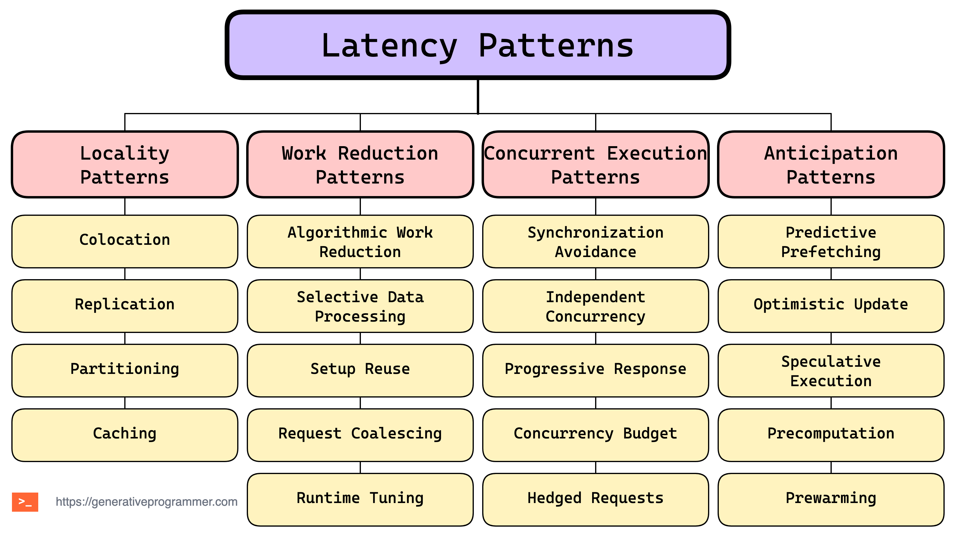
This is why a fast database query or LLM call does not prove that the application is fast. We need to measure the full path as a distribution and identify what controls the percentile we care about. Once we know what dominates the critical path, we can bring requests and data closer, reduce work, execute independent work concurrently, or anticipate predictable work. These are general distributed-system patterns that apply equally to AI applications. The map below adapts latency optimization ideas from Pekka Enberg’s Latency into four practical pattern categories.
An agentic request may cross RAG retrieval, databases, a model gateway, one or more LLMs, MCP or other tool servers, and an orchestration loop. A large part of the latency often comes from the LLM calls, but the model is still only one segment of the path. I covered model-serving optimizations such as quantization, decoding, and server scheduling in this talk and this post. In this post, I explicitly focus on non-model latencies across the application path.
Each category bellow explains the patterns through traditional application examples, then how they apply in an AI application. Taken together, there 19 latency patterns across four categories.
Locality Patterns
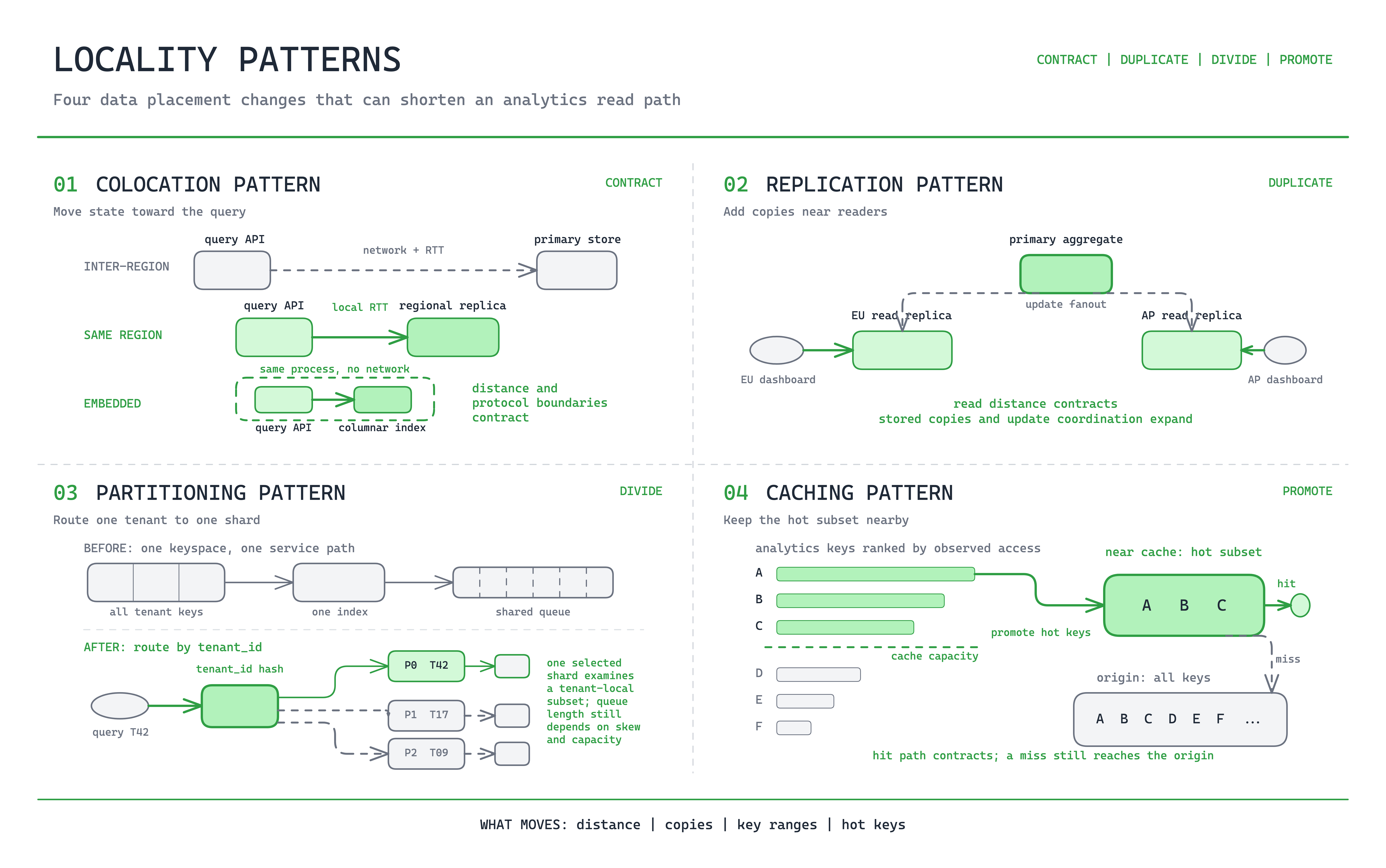
The first thing to check is whether the request and the data it needs are far apart. That distance may be geographical, between services, between processes on one host, or even between a CPU core and memory. There are four common patterns for shortening this part of the path.
1. Colocation Pattern
Colocation shortens or removes a boundary between the source and the target. The scale can vary significantly. A CDN can serve the dashboard shell closer to the user. Application logic can run in the same region as its database instead of crossing a wide-area network. On one host, CPU affinity and NUMA-aware placement can keep hot work and memory near the cores that use them. The mechanism is the same even when the distances are very different.
When to use. Use colocation when the distance between components that frequently interact is a measurable part of the critical path.
The main trade-off. Tighter placement can reduce scheduling flexibility and make failover or scaling across locations more difficult.
2. Replication Pattern
Replication places a readable copy in more than one location. A nearby replica can shorten the read path, but only when the application is allowed to read from it. For example, a dashboard can read tenant data from the nearest regional replica instead of crossing regions for every query.
When to use. Use replication for read-heavy paths that can tolerate a clearly defined level of staleness.
The main trade-off. Synchronous replication may keep the write waiting for required acknowledgements, while asynchronous replication can respond earlier but allow lag. The application must decide which reads can tolerate older data, how they are routed, and what should happen during a failure.
3. Partitioning Pattern
Partitioning divides data or work into units that can be placed and processed independently. It does not make anything closer by itself, but a good partition key can keep a tenant’s query and data together. For example, a dashboard can partition metrics by tenant so that most queries touch one shard rather than several.
When to use. Use partitioning when requests and data share a stable key that can keep related work within one partition or location.
The main trade-off. A poor key can create a hot partition, while a request that spans several partitions brings routing and coordination back onto the critical path.
4. Caching Pattern
Caching creates a shortcut for repeated reads or computation. The hit ratio tells us how often the shortcut works, while the miss penalty tells us how painful the original path remains. For example, a dashboard can cache common aggregates close to the application instead of recalculating them for every page load.
When to use. Use caching when reads or computations repeat and their results can be safely reused.
The main trade-off. A high hit ratio can still produce a bad tail when misses are expensive. Freshness, invalidation, and ownership determine whether the cached result can be trusted.
Choosing What to Bring Closer
In a traditional application, start with the kind of distance that creates the delay. Use colocation when two components communicate frequently, replication when reads are far from the source, partitioning when related data can be kept together, and caching when the same data or computation is requested repeatedly. The patterns can be combined, but each addresses a different reason for travelling across the system.
In an AI application, apply the same test to the orchestrator, the model provider, retrieval store, state store, and tools. Colocate dependencies that communicate frequently, replicate read-heavy knowledge where residency rules allow it, partition state by tenant or session, and cache repeated retrieval, schema discovery, session summarization, policy lookup, or model prefill work.
Work Reduction Patterns
If the latency trace points at computation as the bottleneck, the next move is to remove work. Work that no longer exists cannot delay the request, consume capacity, or create another failure point.
5. Algorithmic Work Reduction Pattern
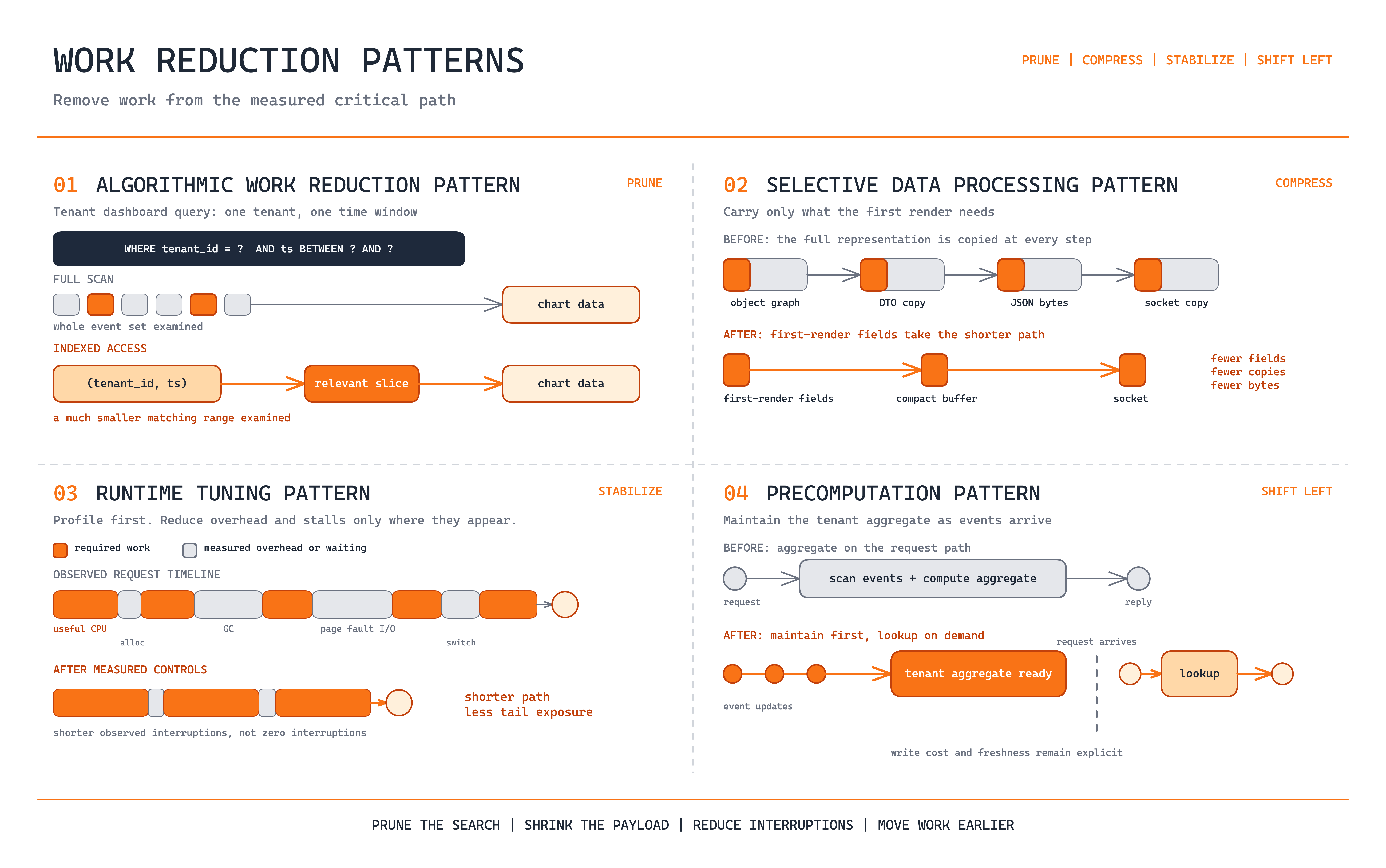
An index over tenant and time can replace a full scan. A hash lookup can replace a linear search. Filtering before an expensive join or sort can reduce the dataset before the costly operation begins. These changes reduce the amount of work rather than making the same work slightly faster.
When to use. Use this pattern when query or computation cost dominates and a better algorithm, index, or data structure can reduce the work.
The main trade-off. A faster access path may require additional indexes, memory, preprocessing, or implementation complexity.
6. Selective Data Processing Pattern
A dashboard does not need the full object graph when the first chart uses five fields. Building large intermediate objects, copying them between layers, serializing them, and then discarding most of the result consumes time without changing what the user sees. A lean response should carry only what the next step needs.
When to use. Use selective data processing when the next step needs only a subset of the available data.
The main trade-off. Removing too much data can trigger another request or prevent a later step from completing.
7. Setup Reuse Pattern
Reusing an established connection, a parsed schema, or validated orchestration state avoids repeating the same setup on every request.
When to use. Use setup reuse when the same initialization cost is paid repeatedly and the resulting state can be retained safely.
The main trade-off. Reused state needs explicit lifecycle, freshness, isolation, and failure handling.
8. Request Coalescing Pattern
Combining several known reads into one request can remove repeated serialization, scheduling, and round trips. This is where request batching can help latency. For example, a dashboard backend can fetch the summary, alerts, and recent events in one call instead of making three sequential requests.
When to use. Use request coalescing when several predictable calls cross the same boundary and can be safely combined.
The main trade-off. A combined request can make one slow operation hold back all the others. It should be measured against the user-visible latency target, not assumed to be faster.
9. Runtime Tuning Pattern
Allocation, garbage collection, demand paging, scheduling, and context switches can all delay useful work. Profile the critical path first, then reduce only the runtime costs that measurably affect it. For example, a service may reduce short-lived allocations or tune its heap after profiles tie p99 spikes to garbage-collection pauses. These costs are measurable suspects, not default explanations for every slow service.
When to use. Use runtime tuning when profiles show that runtime overhead affects the percentile you are trying to improve.
The main trade-off. Runtime tuning can increase implementation complexity and may depend on a specific runtime, operating system, or hardware configuration.
Choosing What Work to Remove
In a traditional application, first identify what kind of work dominates the trace. Algorithmic work reduction changes how the result is found. Selective data processing reduces how much data moves through the path. Setup reuse avoids repeating initialization, while request coalescing removes repeated boundary crossings.
In an AI application, reduce latency by doing less work. Use regular code or indexed search for simple lookups instead of calling a model. Send only relevant information to the model, reuse existing tool connections, and combine calls that always happen together. Use a smaller model for simple tasks when it provides good enough results, stop generation when the answer is complete, and limit how much tool output enters the prompt. But do not remove so much context that the application must fetch more information and call the model again. That extra round trip may make the request slower overall.
Once the remaining work is necessary, the next question is whether it really has to run in sequence.
Concurrent Execution Patterns
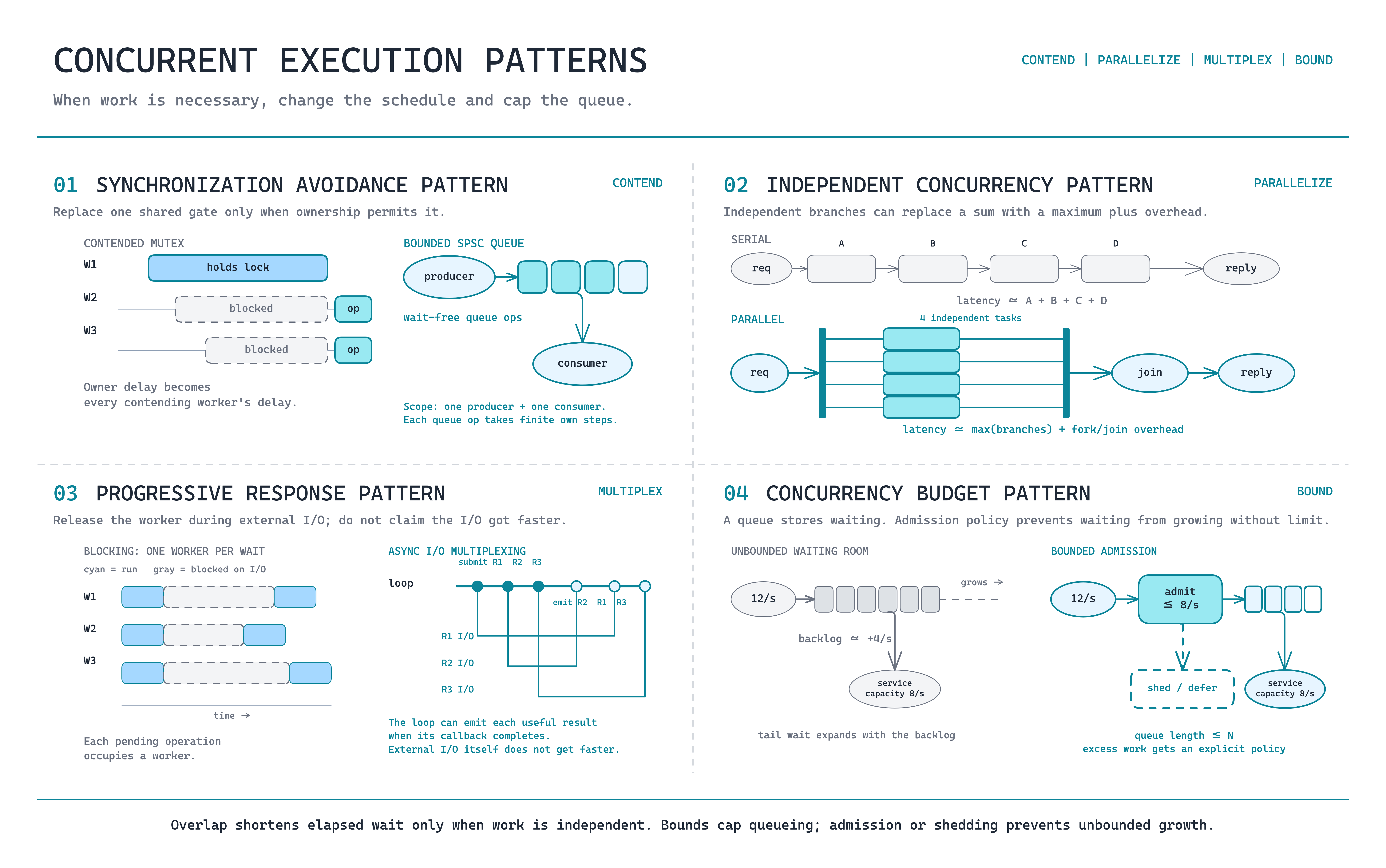
Some work is necessary but does not need to happen in sequence. Suppose authentication must finish first, but four dashboard panels are then independent. Running them serially makes the user wait for roughly the sum of their durations. Starting them together can bring the wait closer to the slowest required panel, plus scheduling and coordination overhead.
10. Synchronization Avoidance Pattern
A contended lock can make otherwise short operations line up behind one owner. Immutable state may remove the shared dependency, while a single-owner design may replace lock contention with an explicit queue. The important question is whether another operation must finish or release something before this one can continue.
When to use. Use synchronization avoidance when coordination over shared state is a measurable source of waiting and the state can be made immutable, partitioned, or owned by one component.
The main trade-off. Removing a lock may move the waiting elsewhere or require a different state-management model.
11. Independent Concurrency Pattern
Concurrency lets several tasks make progress, while parallelism executes work at the same time. For the dashboard, separate panel reads can run concurrently. In an agentic application, a research agent can query independent document stores and market-data sources in parallel, then join the results before synthesis. If one tool needs an identifier returned by another, that dependency remains serial.
When to use. Use independent concurrency when required tasks have no data dependency and the system has enough capacity to run them together.
The main trade-off. Concurrency does not help when one task genuinely needs the result of another, and it can make latency worse when the fan-out exhausts a shared dependency.
12. Progressive Response Pattern
An event loop can use resources more efficiently while external I/O is pending, but it does not make the database, model, or remote service intrinsically faster. The visible latency improves when an AI application streams useful model output or an independently useful tool result instead of holding everything until the full task completes.
When to use. Use a progressive response when a partial result is independently useful and time to first useful result matters to the user.
The main trade-off. This pattern shortens time to first useful result, not full completion, and the client must handle partial or provisional state.
13. Concurrency Budget Pattern
A queue stores waiting; it does not remove it. If arrivals exceed capacity, the queue grows and tail latency follows. Set a concurrency budget, propagate deadlines and cancellation, apply backpressure, and stop work when the user no longer needs it. For example, a dashboard can allow only four panel queries to run at once rather than sending an unbounded fan-out to the database.
When to use. Use a concurrency budget when one request can fan out across services, databases, models, or tools and overload a shared dependency.
The main trade-off. A budget that is too low leaves capacity unused, while one that is too high moves the queue into a downstream dependency.
14. Hedged Requests Pattern
Request hedging reduces exposure to a straggler by sending equivalent copies and accepting the first valid response. For example, after a short delay, a service can send the same read to a second replica and use whichever valid response arrives first.
When to use. Use hedged requests when rare stragglers dominate tail latency, spare capacity exists, and the operation is idempotent or side-effect-free.
The main trade-off. Hedging spends extra capacity and can worsen overload if it is used without a strict budget.
Choosing What Can Run Together
In a traditional application, synchronization avoidance removes unnecessary waiting, while independent concurrency overlaps work that has no dependency. A progressive response changes when useful output becomes visible, not how fast the full operation completes. A concurrency budget protects shared capacity, while hedged requests spend additional capacity to reduce exposure to rare stragglers.
In an AI application, run independent model, tool, and retrieval calls at the same time. If one call needs the result of another, run them in order. Progressive responses, such as streaming, show useful results sooner but do not change which calls can run together. Limit how many model, agent, tool, and retrieval calls run at once to avoid overload. Use hedged requests only for operations that are safe to repeat. The goal is to reduce waiting, not to start as many calls as possible.
Anticipation Patterns
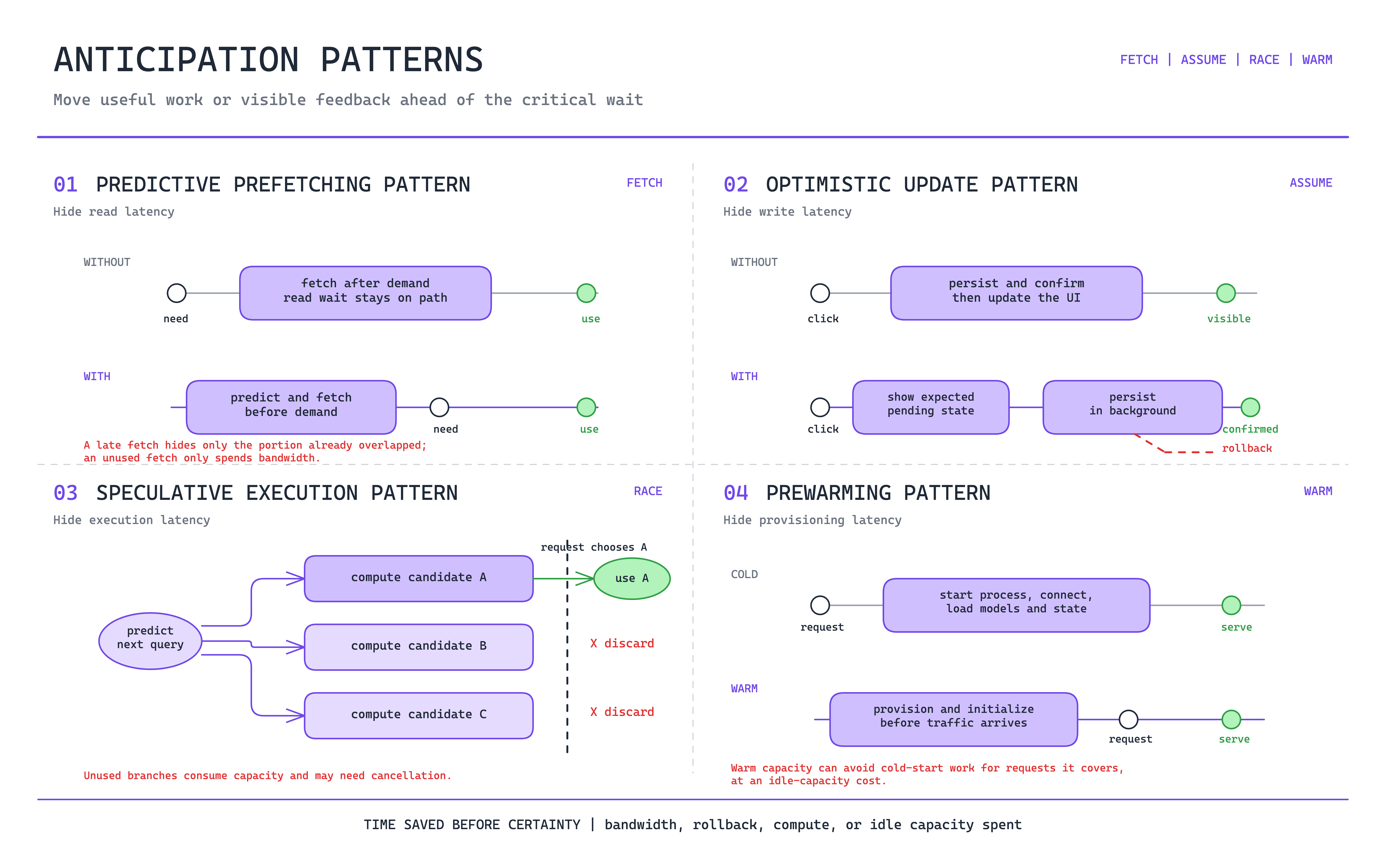
If a remaining delay cannot be removed or safely overlapped after the request arrives, we can anticipate likely work and move it earlier.
15. Predictive Prefetching Pattern
Once authentication identifies the user, the application may fetch the default dashboard before the browser asks for its first panel. This is a prediction about a future read.
When to use. Use predictive prefetching when the next read is predictable enough to justify occasionally wasted work.
The main trade-off. Prefetching helps only when the data arrives in time and is still useful when the application needs it. A wrong prediction consumes resources without shortening the request.
16. Optimistic Update Pattern
A filter can appear selected while persistence continues, as long as the interface shows that the change is pending and can roll it back after a failure. This improves perceived latency after the user acts. It does not make durable completion happen earlier.
When to use. Use optimistic updates when success is common, failure is visible, and the operation can be safely reversed.
The main trade-off. A failed operation requires rollback, and provisional state must never be presented as completed work.
17. Speculative Execution Pattern
Speculative execution runs a likely branch before the actual choice arrives. For example, a dashboard can start calculating the most common time range while the user is still opening the time-range filter.
When to use. Use speculative execution when a small number of likely branches can run safely, independently, and be cancelled.
The main trade-off. The work must be isolated and cancellable because a wrong prediction consumes resources without helping the request.
18. Precomputation Pattern
Maintaining a tenant aggregate as events arrive can replace repeated foreground computation with a read. Precomputation moves known work from the foreground request to the point where the source data changes.
When to use. Use precomputation when an expensive result can be refreshed as its source changes rather than calculated for every request.
The main trade-off. Precomputed results consume storage and refresh capacity, and they may be stale when the source changes faster than they can be updated.
19. Prewarming Pattern
A small worker pool, connection pool, or execution environment can be initialized before traffic arrives. Prewarming moves predictable setup cost off the foreground critical path.
When to use. Use prewarming when cold-start or setup cost is predictable and keeping limited capacity ready is affordable.
The main trade-off. Warm resources consume capacity even when no request uses them.
Choosing What to Do Earlier
In a traditional application, predictive prefetching prepares a likely read, optimistic updates show likely success before durable completion, and speculative execution starts a likely branch. Precomputation prepares reusable results when source data changes, while prewarming prepares resources before requests arrive. The difference is what is moved earlier: data, feedback, a branch, a result, or capacity.
In an AI application, start predictable work early. Once the application understands what the user wants, it can fetch likely context and start safe, read-only searches. It can also prepare reusable data such as embeddings, indexes, summaries, and policy information, or keep agent workers and model or tool connections ready to avoid setup delays. If the interface expects a tool action to succeed, show it as pending until it actually completes.
Measure whether this early work was used, finished in time, and reduced latency. Also track wasted work and actions that had to be reversed. Cancel work when it is no longer needed. If early work consumes enough resources to slow normal requests, it is not an optimization.
Find the Bottleneck, Apply the Pattern
Do not start by choosing a pattern. Start by tracing the full request and locating where delay enters the critical path: context retrieval, model access, tools, agent coordination, or verification and delivery.
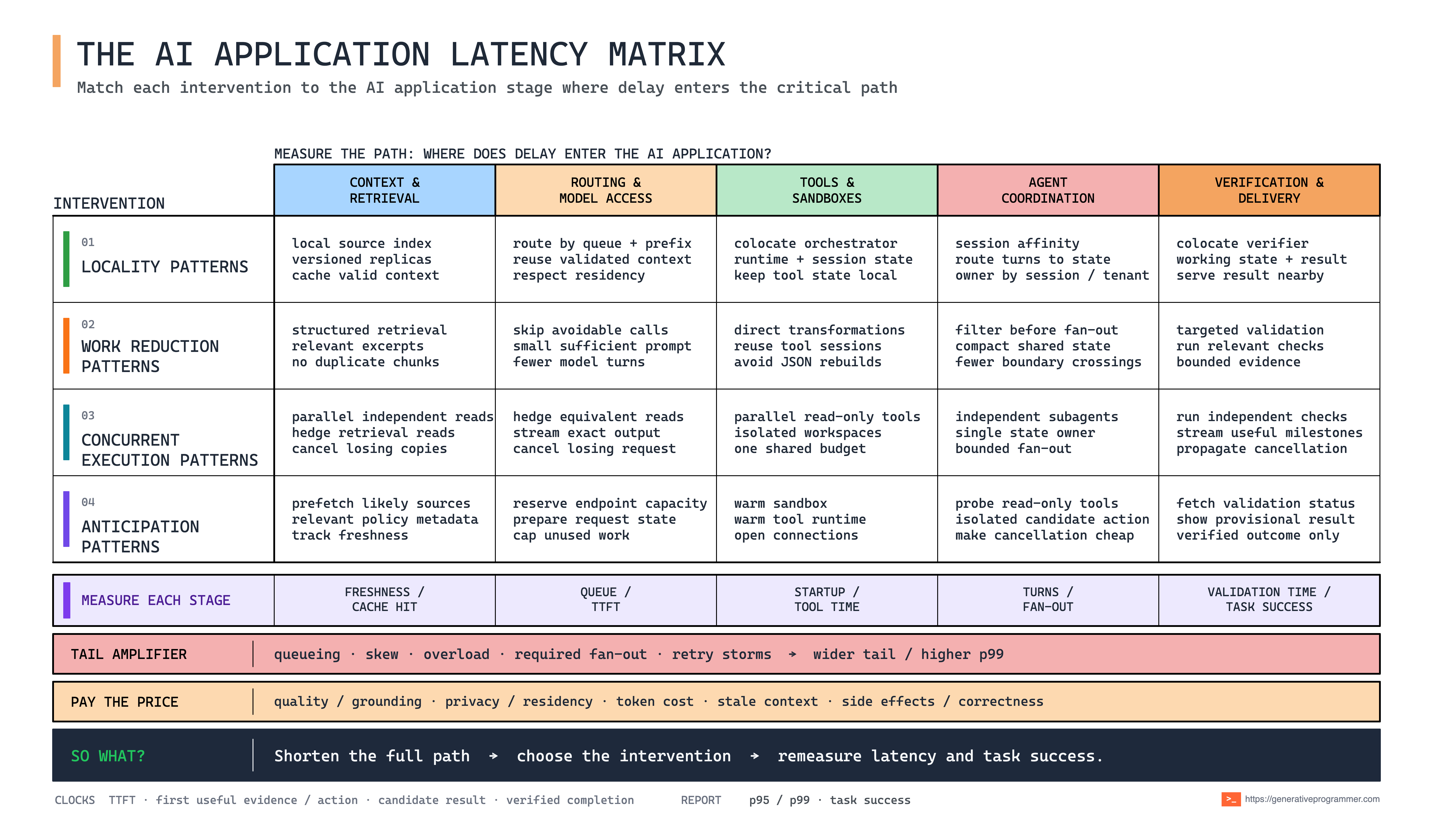
Read the matrix in two moves. First, choose the column where the delay appears. Then move down that column and select the intervention that matches its cause:
Locality Patterns: The request, data, or dependency is too far away.
Work Reduction Patterns: The application performs unnecessary computation, data processing, or calls.
Concurrent Execution Patterns: Independent work is waiting in sequence.
Anticipation Patterns: Predictable work remains on the foreground path.
The cells are starting points, not a checklist. Pick the smallest pattern that changes the dominant part of the path. Before applying it, check whether it will amplify the tail or trade away quality, freshness, privacy, cost, or correctness. Then measure the same latency clock at the target percentile together with task success. If the bottleneck moves, return to the matrix.
Further reading
The following resources cover the main ideas behind this catalogues.
Measuring the AI application path
OpenTelemetry, Generative AI semantic conventions: shared spans, metrics, and events for models, agents, and MCP.
NVIDIA, LLM inference metrics: definitions of time to first token, end-to-end request latency, inter-token latency, and throughput.
Gil Tene, How NOT to Measure Latency: coordinated omission and other measurement errors that can hide real latency.
Fan-out and tail latency
Jeffrey Dean and Luiz André Barroso, The Tail at Scale: why rare stragglers become common as requests fan out.
Marc Brooker, Serial, Parallel, and Quorum Latencies: a simulator for understanding how latency composes across dependent and parallel work.
System-level diagnosis
Pekka Enberg, Latency: Reduce Delay in Software Systems (highly recommended read and the inspiration for this post)
Brendan Gregg, Systems Performance: Enterprise and the Cloud, Second Edition: a methodology for finding latency outliers across the full stack.
Alexey Ivanov, Optimizing web servers for high throughput and low latency: a production case study from hardware and NUMA to the kernel and application.